Best Practices 1 - V488 Sge

[HQA]

Edit 20260906b
Edit 20260907
Edit 20260917
Edit 20260917a
Edit 20260917b
While there are threads in the Community/Alerts forum on various stars, I’d like to open some threads in this forum regarding Best Practices for observing some of these stars. I don’t want to highlight any specific observer, but instead note the observations that a professional might ignore or be concerned about. I hope that everyone has a thick skin and takes these comments constructively. Also note that these comments are mine alone, and do not necessarily reflect the opinion of the AAVSO.

Firstly, those with discrepant measures should NOT just delete them. Find out what is wrong and fix them and resubmit. You’ve spent significant time acquiring the data, analyzing the photometry and submitting your results. Improving that analysis makes your measures useful to the professionals and saves your “investment”!

On each of these Best Practices threads, I’ll edit this original post as new information comes forth.

One such star is V488 Sge, or Nova Sge 2026. This new nova is an important one - easily observed for both northern and southern observers, bright, and with active discussion as to its classification, reddening and the like. Here is the latest light curve:

well, actually not quite the full light curve. The NMW-Texas Tech survey fainter-than results have been added by Kirill Sokolovsky, and while they are unfiltered, they provide excellent historical evidence prior to the outburst.

The LCG plot is cluttered and confusing. Well over half of the data comes from one-shot-color (OSC) or DSLR observers, and at very high cadence. High cadence is useful for typical CV outbursts like WZ Sge stars, where you might see superhumps - but only if the photometric precision is adequate. For these RGB points, I think the photometry is far poorer than the quoted uncertainties, and frankly, I will delete them and not discuss RGB data further. I think the Smart Telescope Working Group will have the definitive analysis software for one-shot-color cameras in the future.

Now, let me highlight some of the discrepant points:

Dataset 1 is important, because it could define when the peak of the outburst took place, if it is real. I have confidence of the prior BVR dataset because I know the observer. The highlighted dataset, though, only has V and comes just 18 minutes before another observer records a V value 0.6magnitude brighter. I consider this fainter measure questionable, but I can’t ignore it either. Another reason why I might question this measure is that there are several measures on this light curve that are significantly fainter than the typical trend. This is why accurate photometry is so important!

Datapoint 2 is a VR set that looks suspiciously faint. The observer has incomplete metadata, not indicating the airmass, check star, chart, etc. and in addition, there are no other observers in the same time interval. Did the nova fade for some reason, or are these real measures? I seriously doubt the latter, as Rc is shown as being fainter than V, which is not physical. Dataset 3 is another where BVR are fainter than I’d expect, and with limited metadata. Datapoint 4, a V measure, has complete metadata, but includes a comment code of B, meaning bright moonlight or sky. There are other observers at the same time that are a half-magnitude brighter.

Dataset 5 is a cluster of V&R measures from the same observer as dataset 2. While they are submitted with uncertainties in the 0.04mag range, it is pretty obvious to me that the true uncertainty is much larger. They are also transformed OSC measures, and as I said before, I just don’t trust such data. Note that there are later datasets from the same observer, with V being more and more deviant. I’m betting some of this is the mismatch between tricolor G and Johnson V, especially when Halph emission is involved. So again, as a professional, I’d delete sets 2 and 5 before any further analysis. Finally, dataset 6 is a B/Rc set with no corresponding V. These measures occur at essentially the same time as another observer, whose data follow the mean curve. Again, the B/Rc pair look suspicious without enough information to keep or discard.

I’ve only highlighted the first few days of the lightcurve. Most of the later light curve has discrepant photometry, mostly from the same observers.

Webobs 2.0, which you are now required to use, shows the lightcurve for the submitted star, and so you can see for yourself when your data does not seem to follow a trend. Don’t just delete the entry and move to the next submission - learn why the photometry might be wrong and apply that lesson to your next submission!

In case you want to see my photometry, I’ve analyzed 5 nights from BSM_NH using VPHOT and submitted the transformed BVRI data under my obscode (HQA). The weather is supposed to be decent over the next week, so I’ll add more BSM_NH observations as they are taken.

My recommendations:

• use webobs 2.0 to ensure your measures fit the existing light curve on a variable. If not, examine your images and/or analysis techniques. If you can’t find an error, then submit your measures, but I normally include a note indicating that you can’t see a problem, so that the researcher knows that you looked. It may be that a star faded or flared and the submission is correct.
• acquire at least 3 datasets per observing session. For example, if you are using BVRI, then take BVRI BVRI BVRI. Form average and standard deviation and submit those averages. This gives far more accurate uncertainty estimates and better magnitudes.
• don’t submit high cadence data unless the variable warrants it. This increases your observing totals, but does not help the researcher or the light curve.
• include as much metadata as possible, especially things like comp star names, airmass, etc. If performing ensemble photometry, put the star names used in the notes field.
• on fading stars like novae, remember to adjust your exposures as the star brightens or fades, and perhaps change comp stars to match the variable star’s brightness.
• on fading stars, watch out for nearby star contamination. That 12th magnitude companion is not important when the nova is at 8th magnitude, but becomes really critical to avoid when the nova fades!
• be really, really careful if you decide to multiplex your images and include photometry for other variables in the field. They need to be properly exposed and you need to examine them for contaminating neighbors too. Those other variables may also be on the edge of your field and suffer residual vignetting or image distortion, making their photometry unreliable. Care is all-important!
• as the nova fades, consider changing your comp stars so that they remain about as bright as the nova. You do not want to use comp stars that are several magnitudes different in brightness.
• Also, keep monitoring the nova even after it fades, and when it returns from behind the Sun. Novae quite often recover in brightness after the initial dust fade, and that late-time behavior is not well-covered. That being said, often the dust fade is followed by a nebular phase that is dominated by emission lines. Your photometry may not transform as well.

I’ve now submitted the most recent BSM_NH2 photometry from 20260906. As you can see, the nova is decreasing smoothly at BVI, but decreasing far more slowly at Rc. This is because of the whopping Halpha emission that almost always appears on novae. This is also one of the reasons I highly recommend multifilter observations of almost all targets. For novae, and especially supernovae, the shapes of the light curve will be different in different passbands, giving astrophysical information. Often even the peak of an outburst will occur at different times. For eclipsing binaries, the depth of the eclipses gives temperature information for the two stars. Exoplanet transit depths are similar in all passbands, but the “transit imposters” will show their differences. And so on - almost every target yields more information with more filters.

I highly recommend reading the paper by Strope, Schaefer and Henden (2010AJ…140…340S) to see the wild variation of novae light curve shapes. Into which class will V488 Sge fit?

T3, when a nova drops by 3 magnitudes from peak, occurred about 10 days after peak, which classifies V488 Sge in the “fast” category. If I were a betting man, I’d say that we should see the dust fade sometime soon. Be prepared for this. A Best Practice is to understand the type of star that you are observing. When the fade happens, you need to quickly adjust your exposure times and pick out new comp stars. Can you monitor the nova during the fade? Very few light curves have such data points. Take really long exposures (an hour is not out of the question) and try to reach those faint regimes. One thing to watch: there are a couple of ~16mag stars about 10arcsec distant towards the west that will make measurement difficult during the fade. Be careful not to measure one of them instead of the nova!

I forgot that I obtained several early datasets from a Spanish telescope. I’ll process those nights soon and submit the results with some more words. I also have photometry from XPASS. It will be interesting to see how those three very different telescopes line up, since all of that data will be transformed and analyzed identically.

Now that the nova has faded to around 11th magnitude, we start running into the issues of Milky Way crowding. Our galactic plane gives us the advantage of having lots of stars, increasing the chance of finding a nova. However, the big disadvantage is the “lots of stars”. While a nova is bright, this is not a consideration. When it fades, you need to know your system’s ability to reject interfering background stars.

Here is a V-band image from 20260911 from XPASS, the 30cm telescope in my backyard. It has the typical 2-3arcsec seeing of sea-level sites in the Northeastern US.

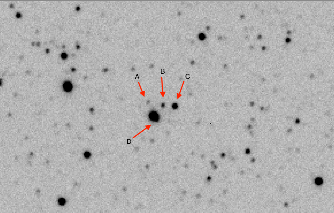
Stars A,B,C are easily seen in this image, and range from about 8arcsec from the target to about 19arcsec. You have to worry particularly about star C, since it is the brightest of the bunch. However, note that the nova itself seems to have an elongated profile. There is actually a nearby star, which I label D. If you want to see the whole setup, here is the Simbad colorized DSS image:

where the nova position is shown with the little box near the center. You can see how these two images relate to one another, and you can see how star D is going to be a problem as the nova fades. In fact, star D is roughly the same brightness as star B, so if we determine star B’s magnitudes, you might be able to use the Nemisis spreadsheet to correct the nova’s brightness. Once the nova fades below about 18th magnitude, we can measure star D’s brightness more accurately. Even then, star D has nearby crud that will interfere.

As a final comment on the crowding issue, here is part of a V-band image from a 50cm telescope for which I am a partner:

The seeing is a bit better, so the nearby companion is readily visible. As you can see right now, the companion is a small fraction of the total flux, but it is probably already contributing a few hundredths of a magnitude of an offset. This will get worse as the nova fades.

So for both novae and supernovae, you have to be careful about the background. I rarely measure supernovae unless they are really on the outskirts of a large galaxy, and I usually put a note in novae photometry submission indicating seeing, aperture size and possible contamination. For most faint nova photometry, I use psf-fitting techniques rather than aperture photometry, in order to reduce background contamination.

[MZK]

Arne:

An observation of the accuracy of some DSLR magnitudes follows: Despite the large scatter of ZZHA’s data, I want to generally observe/hypothesize that the mean magnitude of these time series measurements seem to likely agree quite well with the likely more reliable Johnson Cousins mean BVR light curves. Importantly, these DSLR data probably provide useful data prior to the peak! They also may clearly show a ‘real’ dip at JD 279? I wonder what these DSLR results would look like IF they had been averaged for groups of data points? IF the observer had looked at the Check star scatter, it would have provided a good indication of the real precision of the measurements (standard deviation) and how to improve the target magnitudes. Thoughts?

Ken (MZK)

[HQA]

Hi Ken,
ZZHA’s tricolor observations have ~0.15mag RMS scatter, while the observer reports 0.06-0.08mag or so. This means that the true uncertainty is being underestimated. In addition, the observations are untransformed, and RGB filters have typically huge overlaps and are difficult to compare with the usual Johnson/Cousins. I would have strongly preferred it if the observer had averaged their data rather than submit a thousand-point cloud with larger uncertainty. I tend to downplay such photometry more than I should, but since I don’t fully understand that magnitude system and the methodology, I wait for the Smart Telescope folks to give the definitive answer.

That being said, ZZHA did a number of things MUCH better than the typical CCD/CMOS observer. If you click on any of those observations, the entire ensemble is shown in the notes field, very helpful for researchers. And as you mention, those RGB measures fall on dates where no other observations were being reported, and if you trust them, show changes in the light curve that would have been missed. However, note that the structure of the dip near JD2461279 in G does not match very well the observer’s B data.

The bottom line is that precision matters. With good precision and accuracy, overlap between observers is less important on these stars that are rapidly evolving. The second point is that there are MANY more potential observers with tricolor systems than those with monochrome cameras and filters. The Smart Telescope Working Group is making great headway in understanding tricolor photometry and creating a pipeline to get the maximum accuracy from that data. Until then, I still prefer BVRI!

[Zhang_Jiashuo]

Hi everyone,​
I’m very glad to see this new discussion section.​ In fact, I noticed this discussion page more than ten hours ago, but I did not have enough time at that point to look into it further.​

I think the suggestions from Arne and Ken above are very useful, and they may also be helpful for other observers using color cameras.​

Regarding the brightness decline around JD 2461279, as far as I remember, it was present in all three G, R, and B bands, although at the time I mainly submitted the G-band data.​

However, I noticed something quite interesting. Near the minimum brightness, the G-band data were around magnitude 7.58, while there was a V-band measurement of magnitude 7.60 at JD 2461279.09028. At JD 2461279.26, the G-band brightness was about magnitude 7.35, and some time later another observer reported a value of about magnitude 7.36.​
(It is worth mentioning that the values above are only approximate numbers that I estimated visually on my phone.)​

Considering that these two V-band measurements happen to fall near the minimum and near the point where the brightness recovered, the reality of this brightness decline in the nova now seems somewhat more convincing. Following Ken’s suggestion above, I also made a simple attempt to average the data, and the decline became considerably more apparent.​

Of course, there was also a V-band measurement of magnitude 7.61 at JD 2461278.93741. However, considering Arne’s comments above, I have temporarily ignored this data point.​

Over the next few days, I will try to find some time to analyze these data again and further improve my current measurement procedure. I will also follow the suggestions above and apply more averaging to the data.​

As for some of the data after JD 2461280, since they were not obtained by me, I would prefer not to comment on them before examining them more carefully. However, the effect pointed out by Arne may indeed have played a role. Perhaps, for this type of object, we need to consider the issue of transforming TG measurements to V when using color cameras for photometry during the later stages of the outburst.​

Let’s see what further information the Smart Telescope Working Group can summarize that may be worth discussing.​
@HQA @MZK

Best regards,
Jiashuo（ZZHA）

[HQA]

Thanks for the information, Jiashuo! There was one V-band observation during your dip that I saw, and I had enough doubt regarding it that I did not mention the observation. I was hunting around for corroborative information from a survey without much luck. ASAS-SN did not observe during that day. I don’t know where TESS was pointed, as that survey would of course give exquisite coverage of the peak. Maybe someone can check.

One of the big advantages of OSC/DSLR observing is bringing in so many additional observers who can fill in the light curve. This is strongly visible in your datasets that span groups of CCD/CMOS observers and potentially catch features like that dip. We just need to find ways to make such observations even more scientifically valuable.

Can you give us details of your telescope system? The cadence looks a bit like a Seestar S-50 or other smart telescope.

[Roy_Axelsen_ARX]

When I started into photometry around 20 years ago, the thing that really intrigued me was to understand how accurate measurements in two or more passbands could be made. I pretty soon realized that the key to this was to determine transformed magnitudes, and after that all my DSLR photometry was transformed.

As Arne notes a lot of RGB photometry in the AAVSO database is not transformed. I think I know why this is so - understanding transformation takes a bit of work, and implementation can also be challenging. My attitude is to face the challenge and get the satisfaction from seeing the results.

I may be wrong, but I don’t think there is any easy-to-understand software out there that readily does the transformations for you if you start with DSLR RAW images or maybe even OSC FITS images.

[HQA]

Hi Roy,
The Smart Telescope Working Group is creating a quality pipeline that includes transformation. The basic idea is that some script on the telescope end finds, and does basic photometry of, every star in an image, creating a star list. That list will be uploaded to the AAVSO, where an analysis pipeline does the final photometric steps. I expect a preliminary version of their software (for smart telescopes, at least) to be released in the next 6 months or so. Hopefully it will be extended to work with all OSC/DSLR systems in the future.

I think the concept of a pipeline is the simplest method, and avoids the confusion of a user interface when performing steps like transformation. My own software for monochrome+filter cameras is pipelined and works with starlists in a similar manner, though I do it in several steps with intermediate files so that I can monitor progress.

[HTY]

Following up on the comment above about how it may become more difficult to transform between tricolor G and Johnson V once H-alpha emission is involved: I chased one of my own discrepant points on this nova and would like to share what I found. As a disclaimer, some of my research used AI (Claude Fable 5.1) but I’ve reviewed every word and edited where I thought appropriate.

On the night of August 25-26 the green channel from my one-shot-color Seestar S50, transformed to V with coefficients fitted on Landolt standard fields, gave V = 7.13 - pretty close to other observers but slightly brighter. On the night of September 4-5 the green channel transformed to V gave V = 9.76. My reported values on both of these nights were the means of 12 frames. V measurements with monochrome CCDs that same night of Sept. 4-5 and the next night all fell between 10.06 and 10.51. A second color camera reporting its raw green channel (TG) nine minutes before one of those CCD V points read 9.76 — identical to my “transformed V” and 0.58 mag brighter than the V measured at nearly the same time. My check star agreed with its catalog value to 0.013 mag, and the same two comparison stars gave the monochrome CCD observers their 10.3–10.4. So it was not a zero point error, and it was not a flare. Two types of cameras were simply seeing two different things.

Why transformation cannot fix it. Transformation coefficients describe how a camera’s passband differs from the standard passband for a “normal” star. They are fitted on standard stars, whose light is roughly a smooth continuum. They correct that difference with a color term: “a star this red reads this much different in my green than in V”. That works as long as the target’s spectrum is shaped like the stars the coefficients came from. This nova’s spectrum a couple of weeks past peak is not. The continuous starlight is being increasingly dominated by a handful of emission lines. A color term has no way to know where those lines sit relative to the edges of the two passbands — and that is exactly where the OSC channels and the Johnson/Cousins filters differ:

• the green Bayer channel is wider and bluer than Johnson V; it takes in H-beta (4861 Å) and the strong Fe II lines around 4924–5018 Å that V largely cuts off;
• the red Bayer channel takes in H-alpha (6563 Å) in full, as does Cousins R, but with different weight;
• the blue channel and Johnson B see much the same lines, which is why my B agreed with the CCD B values.

What the spectra show. The spectra posted in the “Possible bright nova in Sagitta” topic are drawn with the star’s continuum flattened to a level of 1, so each line’s height is how many times brighter than the continuum it is at that wavelength. Between 28 August and 4 September:

line	28 Aug	4 Sep	which passband sees it
H-alpha 6563 Å	~4× continuum	~48× continuum	red Bayer channel, Cousins R
H-beta 4861 Å	~6×	~12×	green Bayer channel; only the blue edge of Johnson V
H-gamma, H-delta	3–5×	3–5×	blue channel, Johnson B
Fe II 4924, 5018, 5169, 5317 Å	1.5–3×	1.5–3×	green channel and V
[O III] 4959/5007, [N II] 5755 Å	absent	absent	(the nebular-phase lines; not there yet)

By September 4th the H-alpha line alone carried about as much light as a thousand angstroms of continuum, which is the whole width of a red channel — so a red channel reads the nova far brighter than the continuum would suggest, and the same thing happens to a lesser degree in green through H-beta and Fe II. This is an Fe II-class nova in early decline, not yet in its nebular phase, and it was already enough to put a transformed green channel half a magnitude off Johnson V.

Why the early point was close. In the first days after peak the nova was still continuum-dominated (the “fireball” phase). The spectrum then looked enough like a normal star for the color term to work, and transformed OSC points from that period sit on the CCD curve. The divergence grows as the continuum fades — which is why an observer’s transformed V drifts further from the CCD curve as the weeks pass, exactly as noted above.

I have removed my transformed B/V/R points for the emission-line phase on September 4-5 and resubmitted the same measurements as TG/TB/TR, untransformed, with the ensemble stars and check star named in the notes. They are reported as the original passbands they actually are. The raw channels might hopefully be of some use in a future pipeline.

[1eboeneker]

Thanks for your comments, Arne. They will be taken into account for my next observations.

In regards of your final question… Ssssssomething tellsss me that the classss isss closssse to ssssssometing.

Cheers!

Enrique
BETB

[bskiff]

It is certainly the case that variously weird emission-line objects will not transform accurately (and cannot be). I suspect that proper transformations for the tri-color cameras will require at least bi-color and/or non-linear transformations. Thus the ‘green’ channel transformation might require both B-V and V-Rc colors to transform to standard Johnson V. And depending on how wide the color-range of the standards is, needing a (B-V)^2 term as well would not be surprising.

\Brian

[GFB]

Hi Arne,
I am curious about your use of the starlists. You must have some process to keep track of the objects on each list. Do you import each list to a database of your own for sorting and searching? Would you make a starlist for every exposure in a time series or one giant list for the session?

Bill

[DEY_VAR]

Brian & Timothy,

I don’t believe that you can’t transform pretty much any photometry, continuum only stars to HUGE H-alpha emission objects or even weird emission objects.

If you have determined your filter set transform coefficients from the instrumental system to your favorite standard system and then apply them this nova for example then why is this not sufficient? The transformation process is adjusting for the filter differences only.

Is there some higher order thing going on for say an emission line contained in the edge of your instrumental filter that wouldn’t fall in the standard filter?

Are there any “papers” in the literature concerning this inability to transform a star with emission lines? Be stars, novae, the popular girl T CrB?

There are many sources of errors when playing with DSLR RGB sensors… :It ain’t easy, He’s my bother"! (A play on an olde Hollies tune)

[Roy_Axelsen_ARX]

Jim,

With respect to a classical nova, my understanding (which others will correct if wrong) is that transforming DSLR G to Johnson V is not the problem but transforming DSLR R to Cousins R is. The attached cartoons show why. The vertical red lines were drawn by me to represent the approximate position of the H alpha emission line.

Both DSLR G and Johnson V miss the emission line. Both DSLR R and Cousins R capture the line, which is close to the peak transmission of the Cousins filter, but getting close to the cuttoff of the DSLR filter. Thus the intense H alpha signal will be stronger in Cousins R that DSLR R. You can’t get around that by transforming, (edit) which is based on the continuum of photometric standards and does not include an intense H alpha emission.

[DEY_VAR]

Thanks I already know that, but others may not.

So in classic photometry we should not observe any objects other than those with a flat continuum if we are using non-standard filters such as the much loved Bayer matrix RGB systems.

In my experience observing a few nova over the decades I would argue that you can.

I’ll ask again. Anyone know of an scientific papers that have discussed this theoretically and confirmed with observations that inability? Especially in the case of the Bayer matrix RGB systems.

Please no AI developed answers.

p.s. The B,V,Rc,Ic data shown in LCG-2 as I write can be cleaned up tremendously with a simple removal of one non-AAVSO members data. A few more individual observations could be removed, yes, in that pesky R and even V. What is surprising to me is B looks really good and consistent. What is up with that?

[Roy_Axelsen_ARX]

An example of actual measurements of a nova is shown in Fig. 6.8 of the AAVSO DSLR observing manual. The transformed DSLR R value is substantially (0.4 mag) fainter than the CCD mag.

My comments are related only to novae and specifically to the DSLR R channel.

[TRE]

Roy, your cartoon shows the DSLR passband passes about 35% at the Ha spike while the Rc filter response peaks near Ha. If the sensors ( under the filters ) were equally responsive at just Ha, then a DSLR observer would report a dimmer star. Also the cartoon shows Rc with more bandwidth, so it might be brighter even without the strong hydrogen emission line.

For the Rc on a monochrome camera, we have the manufacturer’s response curve for the camera. We can measure the response curve of the Rc filter or take it from the published specs.

For the DSLR, the published response might be the combination of the pixel plus filter.

I wonder if some of the RGB filter responses could be teased out by comparing (for example) 533mm to a 533mc responses?

Ray

[DEY_VAR]

How does a photometric filter of any sort know what the source of the measured flux comes from in a star being observed? How does it know if the measured flux is from an absorption line(s), flat continuum, or an emission(s) feature in the passband or any combination? It doesn’t.

Oh bother I’m tired… I actually got a few images of olde V488 Sge with a Sony Alpha 6400 and Rokinon 135mm lens from my deck. We shall see what tomorrow brings when I process it thru the Jim manual pipeline! The “coat hanger” in one corner of the FOV makes me remember NQ Vul (N 1976 Vul).

Enjoy the night… I’m not sure we rule it anymore…

[DEY_VAR]

Well I imaged V488 Sge last night using a DSLR and Rokinon 135mm lens, 20x45x stack.

My first comment is that with this and any similar observing setup that the field is very crowded. The nova itself is blended in all the filters, RGB, with the close companion to the NW.

All the comparisons have a least some field-star light contamination in the sky ring. Many comparisons have huge bright stars in any aperture ring size chosen.

If ever there were a great example to use psf fitting and not synthetic aperture photometry this is it.

Got bias in your measures? I know where I’d look first for the source of the bias.

p.s. My data from 2461293.6 was transformed in the standard linear way. Reported as DSLR transformed BVR. Compares favorably to the few CCD obs. around the same time. As expected R is significantly brighter due to the H-Alpha emission in the passband.

[1eboeneker]

Hey everybody!

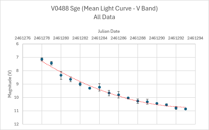
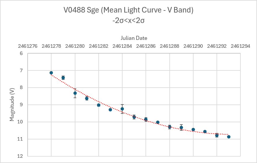
I think this statistical comparison will be interesting for some of you. I have taken from the AID each day’s observations average with the V filter starting August 25 to yesterday.

This graph shows the results averaging each day’s all observations:

This other shows the results not taking into account observations beyond +/- 2 sigma (following somehow the paper that Arne suggested us to read -have you read it already?).

I added to the plots a trendline. According to the aforementioned paper, we can suggest that the shape of both binned light curves corresponds to an S(9) for the moment. We shall see in the future if this classification holds or not. This is why it is important for all of us to keep track of this star, even months or years after its explosion (please read the paper!).

Cheers and behave!

Enrique
BETB

[Roy_Axelsen_ARX]

Jim,

It is worth trying in-focus DSLR images for photometry in crowded fields to reduce the problems you found. A while ago I posted results of a trial of the method. As long as you take multiple images and average the measured mags the results in my hands are as accurate as those with defocussed images. Note that the camera was on a tracking mount.

Here is a copy of most of the post:

It is recommended that photometry with DSLR cameras and one shot colour (OSC) astronomical cameras be performed on defocussed images.

What happens if the recommendation is ignored, and in-focus images are used?

A preliminary look at this with a DSLR camera indicates that photometric accuracy (defined as measured target magnitude minus catalogue magnitude for check stars and photometric standard stars) is as good as it is from defocussed images. Errors for some measurements are < 0.01 mag for transformed V (as is the case for me with defocussed images).

I also obtained one set of transformation coefficients from in focus images which were virtually identical to coefficients from defocussed images. The difference was < 0.01 for Tv_Bv.

However, the standard deviation of a set of measures is higher for in-focus images. That means greater scatter of data in a time series.